Final Report¶

Summary¶

We have implemented a parallelized Poisson image editor with Jacobi method. It can compute results using seven extensions: NumPy, Numba, Taichi, single-threaded c++, OpenMP, MPI, and CUDA. In terms of performance, we have a detailed benchmarking result where the CUDA backend can achieve 31 to 42 times speedup on GHC machines compared to the single-threaded c++ implementation. In terms of user-experience, we have a simple GUI to demonstrate the results interactively, released a standard PyPI package, and provide a website for project documentation.

Source image	Mask image	Target image	Result image

Background¶

Poisson Image Editing¶

Poisson Image Editing is a technique that can fuse two images together without producing artifacts. Given a source image and its corresponding mask, as well as a coordination on the target image, the algorithm always yields amazing result. The general idea is to keep most of gradient in source image unchanged, while matching the boundary of source image and target image pixels.

The gradient per pixel is computed by

\[\nabla(x,y)=4I(x,y)-I(x-1,y)-I(x,y-1)-I(x+1,y)-I(x,y+1)\]

After calculating the gradient in source image, the algorithm tries to solve the following problem: given the gradient and the boundary value, calculate the approximate solution that meets the requirement, i.e., to keep target image’s gradient as similar as the source image.

This process can be formulated as \((4-A)\vec{x}=\vec{b}\), where \(A\in\mathbb{R}^{N\times N}\), \(\vec{x}\in\mathbb{R}^N\), \(\vec{b}\in\mathbb{R}^N\), \(N\) is the number of pixels in the mask, \(A\) is a giant sparse matrix because each line of A only contains at most 4 non-zero value (neighborhood), \(\vec{b}\) is the gradient from source image, and \(\vec{x}\) is the result value.

\(N\) is always a large number, i.e., greater than 50k, so the Gauss-Jordan Elimination cannot be directly applied here because of the high time complexity \(O(N^3)\). People use Jacobi Method to solve the problem. Thanks to the sparsity of matrix \(A\), the overall time complexity is \(O(MN)\) where \(M\) is the number of iteration performed by Poisson image editing. The iterative equation is \(\vec{x}' \leftarrow (A\vec{x}+\vec{b})/4\).

This project parallelizes Jacobi method to speed up the computation. To our best knowledge, there’s no public project on GitHub that implements Poisson image editing with either OpenMP, or MPI, or CUDA. All of them can only handle a small size image workload (link).

PIE Solver¶

We implemented two different solvers: EquSolver and GridSolver.

EquSolver directly constructs the equations \((4-A)\vec{x}=\vec{b}\) by relabeling the pixel, and use Jacobi method to get the solution via \(\vec{x}' \leftarrow (A\vec{x}+\vec{b})/4\).

""" EquSolver pseudocode."""

# pre-process
src, mask, tgt = read_images(src_name, mask_name, tgt_name)
A = build_A(mask)            # shape: (N, 4), dtype: int
X = build_X(tgt, mask)       # shape: (N, 3), dtype: float
B = build_B(src, mask, tgt)  # shape: (N, 3), dtype: float

# major computation, can be parallelized
for _ in range(n_iter):
    X = (X[A[:, 0]] + X[A[:, 1]] + X[A[:, 2]] + X[A[:, 3]] + B) / 4.0

# post-process
out = merge(tgt, X, mask)
write_image(out_name, out)

GridSolver uses the same Jacobi iteration, however, it keeps the 2D structure of the original image instead of relabeling all pixels in the mask. It may have some advantages when the mask region covers the whole image, because in this case GridSolver can save 4 read instructions by calculating the coordinates of the neighborhood directly. Also, if we set the access pattern appropriately (which will be discussed in Section Access Pattern), it has better locality in getting the required data in each iteration.

""" GridSolver pseudocode."""

# pre-process
src, mask, tgt = read_images(src_name, mask_name, tgt_name)
# mask: shape: (N, M), dtype: uint8
grad = calc_grad(src, mask, tgt)  # shape: (N, M, 3), dtype: float
x, y = np.nonzero(mask)  # find element-wise pixel index of mask array

# major computation, can be parallelized
for _ in range(n_iter):
    tgt[x, y] = (tgt[x - 1, y] + tgt[x, y - 1] + tgt[x, y + 1] + tgt[x + 1, y] + grad[x, y]) / 4.0

# post-process
write_image(out_name, tgt)

The bottleneck for both solvers is the for-loop and can be easily parallelized. The implementation detail and parallelization strategies will be discussed in Section Parallelization Strategy.

Method¶

Language and Hardware Setup¶

We start building PIE with the help of pybind11 as we aim to benchmark multiple parallelization methods, including hand-written CUDA code and other 3rd-party libraries such as NumPy.

One of our project goal is to let the algorithm run on any *nix machine and can have a real-time interactive result demonstration. For this reason, we didn’t choose a supercomputing cluster as our hardware setup. Instead, we choose GHC machine to develop and measure the performance, which has 8x i7-9700 CPU cores and an Nvidia RTX 2080Ti.

Access Pattern¶

For EquSolver, we can reorganize the order of pixels to obtain better locality when performing parallel operations. Specifically, we can divide all pixels into two folds by (x + y) % 2. Here is a small example:

# before
x1   x2   x3   x4   x5
x6   x7   x8   x9   x10
x11  x12  x13  x14  x15
...

# reorder
x1   x10  x2   x11  x3
x12  x4   x13  x5   x14
x6   x15  x7   x16  x8
...

This results in a tighter relationship between the 4 neighbors of each pixel. The ideal access pattern is to iterate over these two groups separately, i.e.

for _ in range(n_iter):
    parallel for i in range(1, p):
        # i < p, neighbor >= p
        x_[i] = calc(b[i], neighbor(x, i))

    parallel for i in range(p, N):
        # i >= p, neighbor < p
        x[i] = calc(b[i], neighbor(x_, i))

Unfortunately, we only observe a clear advantage with OpenMP EquSolver. For other backend, the sequential ID assignment is much better than reordering. See the section Parallelization Strategy - OpenMP for a related discussion.

For GridSolver, since it retains most of the 2D structure of the image, we can use block-level access pattern instead of sequential access pattern to improve cache hit rate. Here is a Python pseudocode to show how it works:

N, M = tgt.shape[:2]
# here is a sequential scan:
parallel for i in range(N):
    parallel for j in range(M):
        if mask[i, j]:
            tgt_[i, j] = calc(grad[i, j], neighbor(tgt, i, j))
# however, we can use block-level access pattern to improve the cache hit rate:
parallel for i in range(N // grid_x):
    parallel for j in range(M // grid_y):
        # the grid size is (grid_x, grid_y)
        for x in range(i * grid_x, (i + 1) * grid_x):
            for y in range(j * grid_y, (j + 1) * grid_y):
                if mask[x, y]:
                    tgt_[x, y] = calc(grad[x, y], neighbor(tgt, x, y))

Synchronization vs Converge Speed¶

Since Jacobi Method is an iterative method for solving matrix equations, there is a trade-off between the quality of solution and the frequency of synchronization.

Non-shared Memory Programming Model¶

The above approach works for shared memory programming models such as OpenMP and CUDA. However, for non-shared memory programming models such as MPI, the above approach cannot work well. The solution will be discussed in Section Parallelization Strategy - MPI.

Parallelization Strategy¶

This section will cover the implementation detail with three different backend (OpenMP/MPI/CUDA) and two different solvers (EquSolver/GridSolver).

OpenMP¶

As mentioned before, OpenMP EquSolver first divides the pixels into two folds by (x + y) % 2, then parallelizes per-pixel iteration inside a group in each step.

This strategy can utilize the thread-local assessment as the position of four neighborhood become closer. However, it requires the entire array to be processed twice because of the division. In some cases, such as CUDA, this approach introduces an overhead that exceeds the original computational cost. However, in OpenMP, it has a significant runtime improvement.

OpenMP GridSolver assigns equal amount of blocks to each thread, with size (grid_x, grid_y) per block. Each thread simply iterates all pixels in each block independently.

We use static assignment for both solvers to minimize the overhead of runtime task allocation, since the workload is uniform per pixel/grid.

MPI¶

MPI cannot use the shared memory program model. We need to reduce the amount of data communicated, while maintaining the quality of the solution.

Each MPI process is responsible for only a portion of the computation and synchronizes with other process per mpi_sync_interval steps, denoted as \(S\) in this section. When \(S\) is too small, the synchronization overhead dominates the computation; when \(S\) is too large, each process computes the solution independently without global information, therefore the quality of the solution gradually deteriorates.

For MPI EquSolver, it’s hard to say which part of the data should be exchanged to other process, since it relabels all pixels at pre-process stage. We assign an equal number of equations to each process and use MPI_Bcast to force synchronization of all data per \(S\) iteration.

MPI GridSolver uses line partition: process i exchanges its first and last line data with process i-1 and i+1 separately per \(S\) iterations. This strategy has a continuous memory layout, thus has less overhead compared to block-level partition.

The workload per pixel is small and fixed. In fact, this type of workload is not suitable for MPI.

CUDA¶

The strategy used on the CUDA backend is quite similar to OpenMP.

CUDA EquSolver performs equation-level parallelization. It has sequential labels per pixel instead of dividing into two folds as OpenMP does. Each block is assigned with an equal number of equations to execute Jacobi Method independently. The threads in a block iterate over only a single equation. We also tested the shared memory kernel, but it’s much slower than non-shared memory version.

For GridSolver, each grid with size (grid_x, grid_y) will be in the same block. The threads in a block iterates over a single pixel only.

There are no barriers during the iteration of both solvers. The reason has been discussed in Section Share Memory Programming Model.

Experiments¶

Experiment Setting¶

Hardware and Software¶

We use GHC83 to run all of the following experiments. Here is the hardware and software configuration:

OS: Red Hat Enterprise Linux Workstation 7.9 (Maipo)
CPU: 8x Intel(R) Core(TM) i7-9700 CPU @ 3.00GHz
GPU: GeForce RTX 2080 8G
Python: 3.6.8
Python package version:
- numpy==1.19.5
- opencv-python==4.5.5.64
- mpi4py==3.1.3
- numba==0.53.1
- taichi==1.0.0

Data¶

We generate 10 images for benchmarking performance, 5 square and 5 circle. The script is tests/data.py. You can find the detail information in this table:

ID	Size	# pixels	# unmasked pixels
square6	66x66	4356	4356
square7	130x130	16900	16900
square8	258x258	66564	66564
square9	514x514	264196	264196
square10	1026x1026	1052676	1052676
circle6	74x74	5476	4291
circle7	146x146	21316	16727
circle8	290x290	84100	66043
circle9	579x579	335241	262341
circle10	1157x1157	1338649	1049489

We try to keep the number of unmasked pixels of circleX and squareX to be the same level. For EquSolver there’s no difference, but for GridSolver it cannot be ignored, since it needs to process all pixels no matter it is masked.

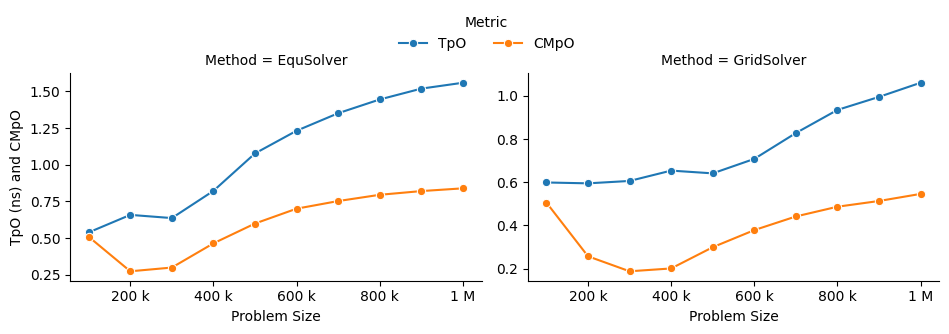
Metric¶

We measure the performance by “Time per Operation” (TpO for short) and “Cache Miss per Operation” (CMpO for short). TpO is derived by total time / total number of iteration / number of pixel. The smaller the TpO, the more efficient the parallel algorithm will be. CMpO is derived by total cache miss / total number of iteration / number of pixel.

Result and Analysis¶

We use all seven backend to run benchmark experiments. GCC (single-threaded C++ implementation) is the baseline. Details of the following experiment (commands and tables) can be found on Benchmark page. For the sake of simplicity, we only demonstrate the plot in the following sections. Most plots are in logarithmic scale.

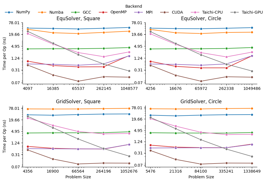
EquSolver vs GridSolver¶

If GridSolver’s parameters grid_x and grid_y are carefully tuned, in most cases it can perform better than EquSolver in a handwritten backend configuration (OpenMP/MPI/CUDA). The analysis will be performed in the following sections. However, it is difficult to say which one is better using other third-party backends. This may be due to the internal design of these libraries.

Analysis for 3rd-party Backend¶

NumPy¶

NumPy is 10~11x slower than GCC with EquSolver, and 8~9x slower than GCC with GridSolver. This result shows that the overhead of the NumPy solver is non-negligible. Each iteration requires repeated data transfers between C and Python and the creation of some temporary arrays to compute the results. Even if we have used vector operations in all the computations, it cannot take advantage of the memory layout.

Numba¶

Numba is a just-in-time compiler for numerical functions in Python. For EquSolver, Numba is about twice as fast as NumPy; however, for GridSolver, Numba is about twice as slow as NumPy. This result suggests that Numba does not provide a general speedup for any NumPy operations, not to mention that it is still slower than GCC.

Taichi¶

Taichi is an open-source, imperative, parallel programming language for high-performance numerical computation. If we use Taichi with small size input images, it does not get much benefit. However, when increasing the problem size to a very large scale, the advantage becomes much clear. We think it is because the pre-processing step in Taichi is a non-negligible overhead.

On the CPU backend, EquSolver is faster than GCC, while GridSolver performs almost as well as GCC. This shows the access pattern largely affects the actual performance.

On the GPU backend, although the TpO is twice as slow as CUDA with extremely large-scale input, it is still faster than other backends. We are quite interested in other 3rd-party GPU solution’s performance, and leave it as future work.

Analysis for Non 3rd-party Backend¶

OpenMP and MPI can achieve almost the same speed, but MPI’s converge speed is slower because of the synchronization trade-off. CUDA is the fastest in all conditions.

OpenMP¶

EquSolver is 8~9x faster than GCC; GridSolver is 6~7x faster than GCC. However, there is a huge performance drop when the problem size is greater than 1M for both two solvers. The threshold is 300k ~ 400k for EquSolver and 500k ~ 600k for GridSolver. We suspect that is because of cache-miss, confirmed by the following numerical result:

OpenMP	# of pixels	100000	200000	300000	400000	500000	600000	700000	800000	900000	1000000
EquSolver	Time (s)	0.1912	0.3728	0.6033	1.073	2.0081	3.4242	4.1646	5.6254	6.2875	7.6159
EquSolver	TpO (ns)	0.3824	0.3728	0.4022	0.5365	0.8032	1.1414	1.1899	1.4063	1.3972	1.5232
EquSolver	CMpO	0.0341	0.0201	0.1104	0.3713	0.5799	0.6757	0.7356	0.8083	0.8639	0.9232
GridSolver	Time (s)	0.2870	0.5722	0.8356	1.1321	1.4391	2.2886	3.0738	4.1967	5.5097	6.0635
GridSolver	TpO (ns)	0.5740	0.5722	0.5571	0.5661	0.5756	0.7629	0.8782	1.0492	1.2244	1.2127
GridSolver	CMpO	0.0330	0.0174	0.0148	0.0522	0.1739	0.3346	0.3952	0.4495	0.5132	0.5394

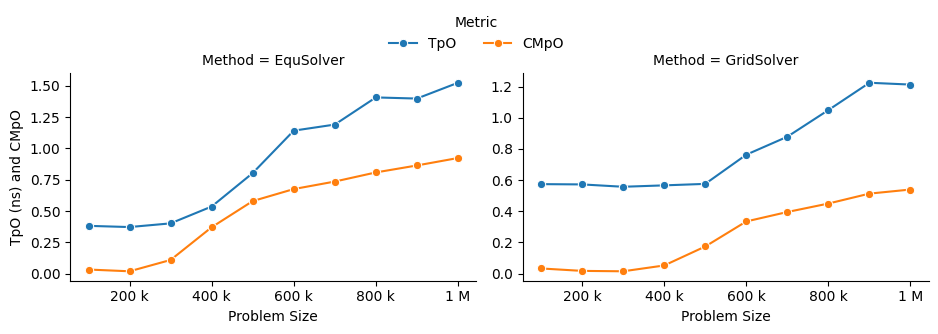
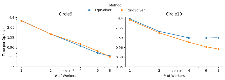
We also investigated the impact of the number of threads on the performance of the OpenMP backend. There is a linear speedup when the aforementioned cache-miss problem does not occur; when the cache-miss problem is encountered, its performance rapidly saturates, especially for EquSolver. We believe the reason behind is that GridSolver can take better advantage of locality compared to EquSolver, since it has no relabeling pixel process and keep all of the 2D information.

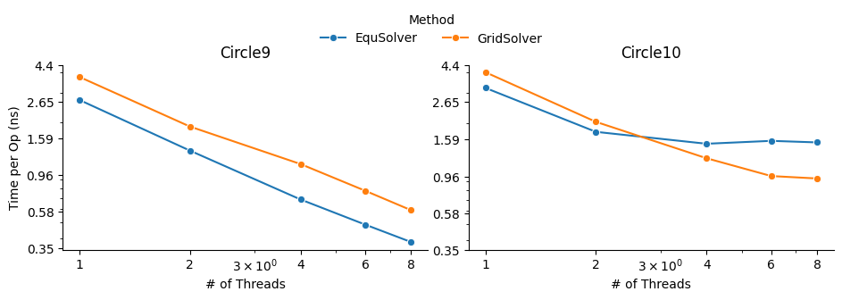
MPI¶

EquSolver and GridSolver is 6~7x faster than GCC. Like OpenMP, there is a huge performance drop. The threshold is 300k ~ 400k for EquSolver and 400k ~ 500k for GridSolver. Fortunately, the following table and plot confirms our assumption of cache-miss:

MPI	# of pixels	100000	200000	300000	400000	500000	600000	700000	800000	900000	1000000
EquSolver	Time (s)	0.2696	0.6584	0.9549	1.6435	2.6920	3.6933	4.7265	5.7762	6.8305	7.7894
EquSolver	TpO (ns)	0.5392	0.6584	0.6366	0.8218	1.0768	1.2311	1.3504	1.4441	1.5179	1.5579
EquSolver	CMpO	0.5090	0.2743	0.2998	0.4646	0.5995	0.7006	0.7525	0.7951	0.8204	0.8391
GridSolver	Time (s)	0.2994	0.5948	0.9088	1.3075	1.6024	2.1239	2.8969	3.7388	4.4776	5.3026
GridSolver	TpO (ns)	0.5988	0.5948	0.6059	0.6538	0.6410	0.7080	0.8277	0.9347	0.9950	1.0605
GridSolver	CMpO	0.5054	0.2570	0.1876	0.2008	0.2991	0.3783	0.4415	0.4866	0.5131	0.5459

A similar phenomenon occurs on the MPI backend when the number of processes changes:

CUDA¶

EquSolver is 27~44x faster than GCC; GridSolver is 38~42x faster than GCC. The performance is consistent across different input sizes.

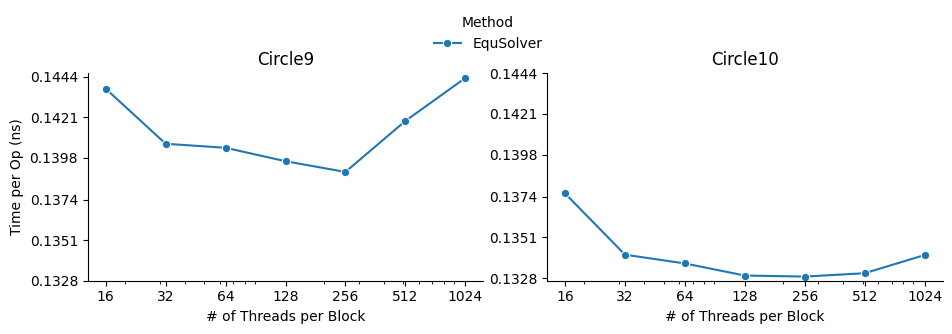
We investigated the impact of different block size on CUDA EquSolver. For a better demonstration, we didn’t use GridSolver because it requires tuning two parameters grid_x and grid_y. By increasing the block size, the performance improves first, reaches a peak, and finally drops. The best configuration is block size = 256.

When the block size is too small, it will use more grids for computation and therefore the overhead of communication across grids will increase. When the block size is too large, the cache invalidation problem dominates, even though fewer grids are used – since we are not using shared memory in this CUDA kernel and there are no barriers to calling this kernel, we suspect that the program will often read values that cannot be cached and will also often write values to invalidate the cache.

Contribution¶

Each group member’s contributions are on GitHub.

REFERENCE¶

[1] Pérez, Patrick, Michel Gangnet, and Andrew Blake. “Poisson image editing.” ACM SIGGRAPH 2003 Papers. 2003. 313-318.

[2] Jacobi Method, https://en.wikipedia.org/wiki/Jacobi_method

[3] Harris, Charles R., et al. “Array programming with NumPy.” Nature 585.7825 (2020): 357-362.

[4] Lam, Siu Kwan, Antoine Pitrou, and Stanley Seibert. “Numba: A llvm-based python jit compiler.” Proceedings of the Second Workshop on the LLVM Compiler Infrastructure in HPC. 2015.

[5] Hu, Yuanming, et al. “Taichi: a language for high-performance computation on spatially sparse data structures.” ACM Transactions on Graphics (TOG) 38.6 (2019): 1-16.

Final Report¶

Summary¶

Background¶

Poisson Image Editing¶

PIE Solver¶

Method¶

Language and Hardware Setup¶

Access Pattern¶

Synchronization vs Converge Speed¶

Share Memory Programming Model¶

Non-shared Memory Programming Model¶

Parallelization Strategy¶

OpenMP¶

MPI¶

CUDA¶

Experiments¶

Experiment Setting¶

Hardware and Software¶

Data¶

Metric¶

Result and Analysis¶

EquSolver vs GridSolver¶

Analysis for 3rd-party Backend¶

NumPy¶

Numba¶

Taichi¶

Analysis for Non 3rd-party Backend¶

OpenMP¶

MPI¶

CUDA¶

Contribution¶

REFERENCE¶