Get Start
Installation
Linux/macOS
# install cmake >= 3.5
# if you don't have sudo (like GHC), install cmake from source
# on macOS, type `brew install cmake`
$ pip install fpie

# or install from source
$ pip install .
Extensions
We provide 8 backends:
NumPy,
pip install numpy;Numba,
pip install numba;GCC, needs cmake and gcc;
OpenMP, needs cmake and gcc (on macOS you need to change clang to gcc-11);
CUDA, needs nvcc;
ROCm/HIP (the CUDA backend on AMD GPUs), needs a ROCm toolchain (
pip install ., or cmake-DUSE_HIP=ON);MPI, needs mpicc (on macOS:
brew install open-mpi) andpip install mpi4py;Taichi,
pip install taichi.
Please refer to Backend for various usages.
After installation, you can use --check-backend option to verify:
$ fpie --check-backend
['numpy', 'numba', 'taichi-cpu', 'taichi-gpu', 'gcc', 'openmp', 'mpi', 'cuda']
The above output shows all extensions have successfully installed.
Usage
We have prepared the test suite to run:
$ cd tests && ./data.py
This script will download 8 tests from GitHub, and create 10 images for benchmarking (5 circle, 5 square). To run:
$ fpie -s test1_src.jpg -m test1_mask.jpg -t test1_tgt.jpg -o result1.jpg -h1 -150 -w1 -50 -n 5000 -g max
$ fpie -s test2_src.png -m test2_mask.png -t test2_tgt.png -o result2.jpg -h1 130 -w1 130 -n 5000 -g src
$ fpie -s test3_src.jpg -m test3_mask.jpg -t test3_tgt.jpg -o result3.jpg -h1 100 -w1 100 -n 5000 -g max
$ fpie -s test4_src.jpg -m test4_mask.jpg -t test4_tgt.jpg -o result4.jpg -h1 100 -w1 100 -n 5000 -g max
$ fpie -s test5_src.jpg -m test5_mask.png -t test5_tgt.jpg -o result5.jpg -h0 -70 -w0 0 -h1 50 -w1 0 -n 5000 -g max
$ fpie -s test6_src.png -m test6_mask.png -t test6_tgt.png -o result6.jpg -h1 50 -w1 0 -n 5000 -g max
$ fpie -s test7_src.jpg -t test7_tgt.jpg -o result7.jpg -h1 50 -w1 30 -n 5000 -g max
$ fpie -s test8_src.jpg -t test8_tgt.jpg -o result8.jpg -h1 90 -w1 90 -n 10000 -g max
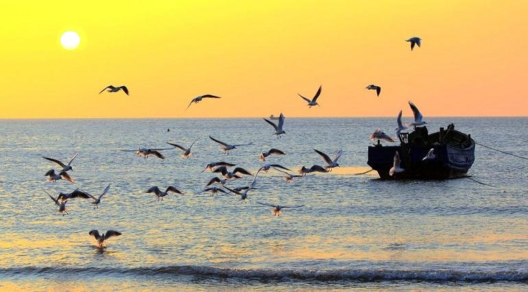
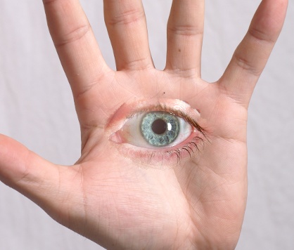
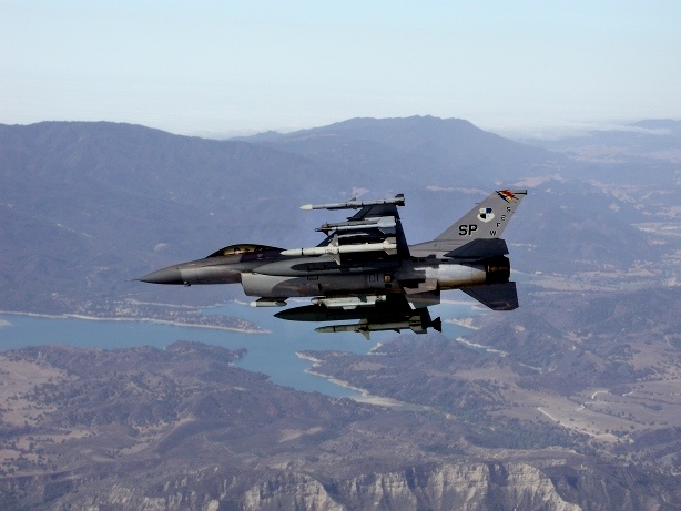
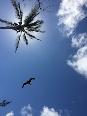
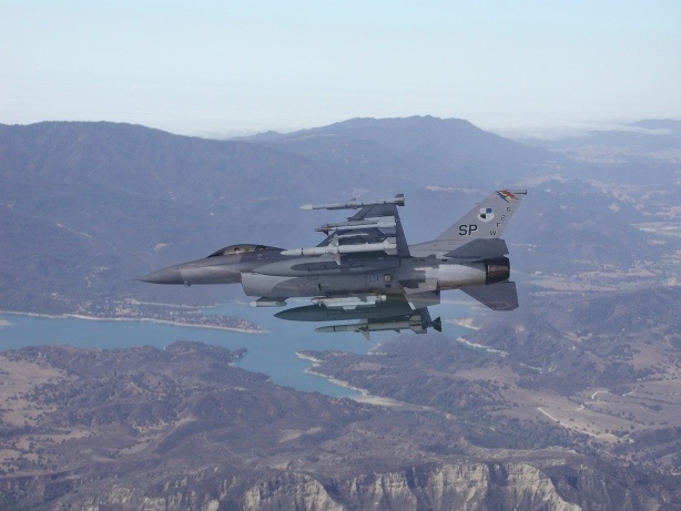
Here are the results:
# |
Source image |
Mask image |
Target image |
Result image |
|---|---|---|---|---|
1 |
|
|
|
|
2 |
|
|
|
|
3 |
|
|
|
|
4 |
|
|
|
|
5 |
|
|
|
|
6 |
|
|
|
|
7 |
|
/ |
|
|
8 |
|
/ |
|
|


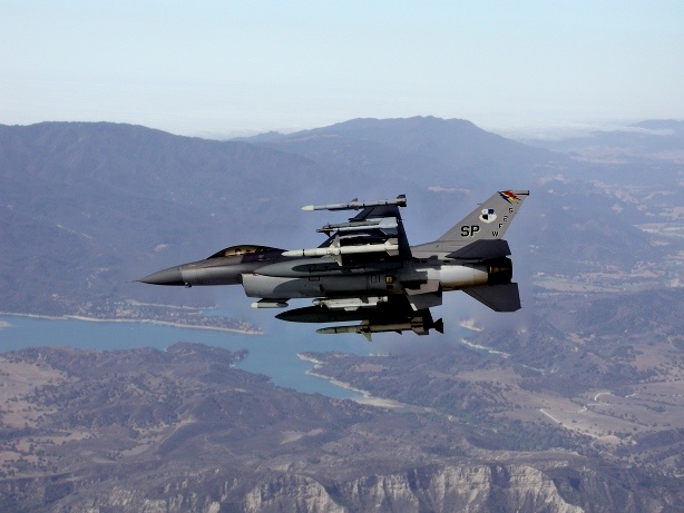
GUI
$ fpie-gui -s test3_src.jpg -t test3_tgt.jpg -o result.jpg -b cuda -n 10000
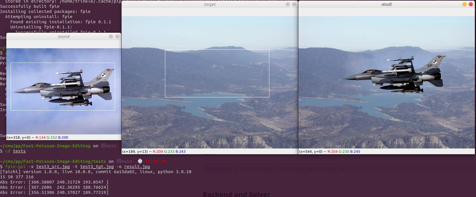
We provide a simple GUI for real-time seamless cloning. You need to use your mouse to draw a rectangle on top of the source image, and click a point in target image. After that the result will automatically be generated. In the end, you can press ESC to terminate the program.
Backend and Solver
We have provided 7 backends. Each backend has two solvers: EquSolver and GridSolver. You can find the difference between these two solvers in the next section.
For different backend usage, please check out the related documentation under docs/backend.md.
For other usage, please run fpie -h or fpie-gui -h to see the
hint.
$ fpie -h
usage: fpie [-h] [-v] [--check-backend] [-b {numpy,numba,taichi-cpu,taichi-gpu,gcc,openmp,mpi,cuda}] [-c CPU] [-z BLOCK_SIZE]
            [--method {equ,grid}] [-s SOURCE] [-m MASK] [-t TARGET] [-o OUTPUT] [-h0 H0] [-w0 W0] [-h1 H1] [-w1 W1] [-g {max,src,avg}]
            [-n N] [-p P] [--mpi-sync-interval MPI_SYNC_INTERVAL] [--grid-x GRID_X] [--grid-y GRID_Y]

optional arguments:
  -h, --help            show this help message and exit
  -v, --version         show the version and exit
  --check-backend       print all available backends
  -b {numpy,numba,taichi-cpu,taichi-gpu,gcc,openmp,mpi,cuda}, --backend {numpy,numba,taichi-cpu,taichi-gpu,gcc,openmp,mpi,cuda}
                        backend choice
  -c CPU, --cpu CPU     number of CPU used
  -z BLOCK_SIZE, --block-size BLOCK_SIZE
                        cuda block size (only for equ solver)
  --method {equ,grid}   how to parallelize computation
  -s SOURCE, --source SOURCE
                        source image filename
  -m MASK, --mask MASK  mask image filename (default is to use the whole source image)
  -t TARGET, --target TARGET
                        target image filename
  -o OUTPUT, --output OUTPUT
                        output image filename
  -h0 H0                mask position (height) on source image
  -w0 W0                mask position (width) on source image
  -h1 H1                mask position (height) on target image
  -w1 W1                mask position (width) on target image
  -g {max,src,avg}, --gradient {max,src,avg}
                        how to calculate gradient for PIE
  -n N                  how many iteration would you perfer, the more the better
  -p P                  output result every P iteration
  --mpi-sync-interval MPI_SYNC_INTERVAL
                        MPI sync iteration interval
  --grid-x GRID_X       x axis stride for grid solver
  --grid-y GRID_Y       y axis stride for grid solver
Benchmark Result
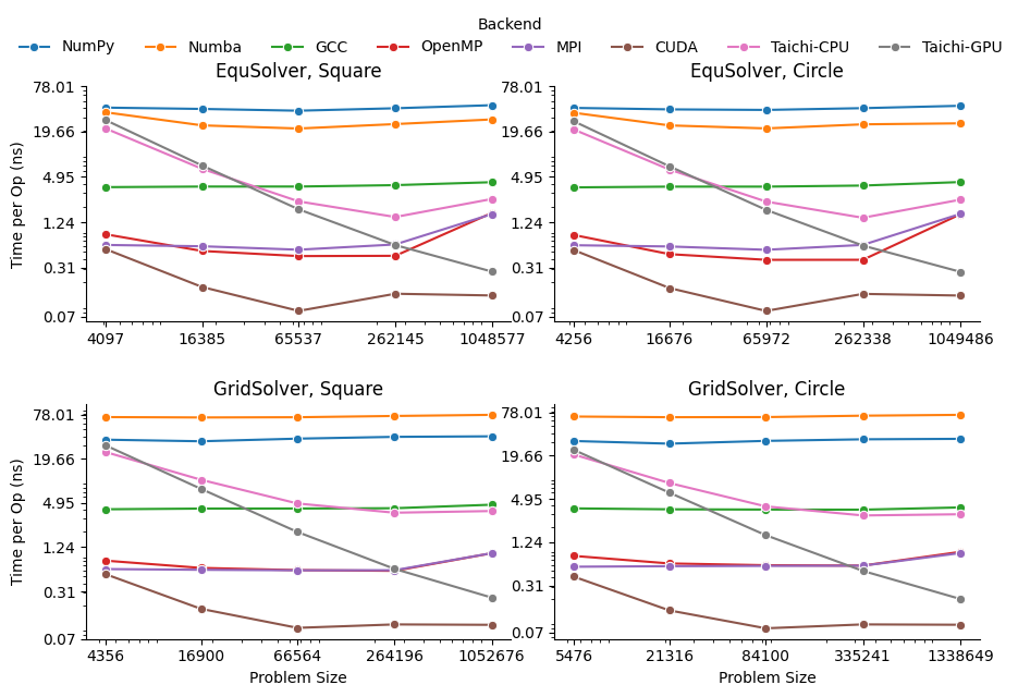
Please refer to Benchmark for detail.
Algorithm Detail
The general idea is to keep most of gradient in source image, while matching the boundary of source image and target image pixels.
The gradient is computed by
\(\nabla(x,y)=4I(x,y)-I(x-1,y)-I(x,y-1)-I(x+1,y)-I(x,y+1)\)
After computing the gradient in source image, the algorithm tries to solve the following problem: given the gradient and the boundary value, calculate the approximate solution that meets the requirement, i.e., to keep target image’s gradient as similar as the source image.
This process can be formulated as \((4-A)\vec{x}=\vec{b}\), where \(A\in\mathbb{R}^{N\times N}\), \(\vec{x}\in\mathbb{R}^N\), \(\vec{b}\in\mathbb{R}^N\), \(N\) is the number of pixels in the mask, \(A\) is a giant sparse matrix because each line of A only contains at most 4 non-zero value (neighborhood), \(\vec{b}\) is the gradient from source image, and \(\vec{x}\) is the result value.
\(N\) is always a large number, i.e., greater than 50k, so the Gauss-Jordan Elimination cannot be directly applied here because of the high time complexity \(O(N^3)\). People use Jacobi Method to solve the problem. Thanks to the sparsity of matrix A, the overall time complexity is \(O(MN)\) where \(M\) is the number of iteration performed by poisson image editing.
This project parallelizes Jacobi method to speed up the computation. To our best knowledge, there’s no public project on GitHub that implements poisson image editing with either OpenMP, or MPI, or CUDA. All of them can only handle a small size image workload.
EquSolver vs GridSolver
Usage: --method {equ,grid}
EquSolver directly constructs the equations \((4-A)\vec{x}=\vec{b}\) by re-labeling the pixel, and use Jacobi method to get the solution via \(\vec{x}'=(A\vec{x}+\vec{b})/4\).
GridSolver uses the same Jacobi iteration, however, it keeps the 2D structure of the original image instead of re-labeling the pixel in the mask. It may take some advantage when the mask region covers all of the image, because in this case GridSolver can save 4 read instructions by directly calculating the neighborhood’s coordinate.
If the GridSolver’s parameter is carefully tuned (--grid-x and
--grid-y), it can always perform better than EquSolver with
different backend configuration.
Gradient for PIE
Usage: -g {max,src,avg}
The PIE paper states some variant of gradient calculation such as Equ. 12: using the maximum gradient to perform “mixed seamless cloning”. We also provide such an option in our program:
src: only use the gradient from source imageavg: use the average gradient of source image and target imagemax: use the max gradient of source and target image
The following example shows the difference between these three methods:
# |
target image |
–gradient=src |
–gradient=avg |
–gradient=max |
|---|---|---|---|---|
3 |
|
|
|
|
4 |
|
|
|
|
8 |
|
|
|
|
15-618 Course Project Final Report
Please refer to Final Report.